Posts

Showing posts with the label Excel

Add a watermark to Office files, Word, Excel, and PowerPoint
Image
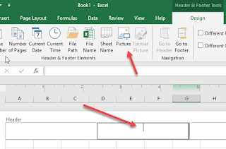
Only Microsoft Word has a built-in watermark feature, but Excel and PowerPoint have a reasonable workaround to adding watermarks on those files, as well. For each of the instructions, I'm using Office 2016 for Windows. Word Word is very easy -- just 3 quick steps. Go to the Design ribbon in your Word document. Click on the Watermark icon of text found near the right end of the ribbon in the Page Background section. Select a watermark you prefer or Custom Watermark... from the menu. If you select the custom option, you have multiple options beyond just custom text. Enter watermark text (or alternatively a picture). Change the font used. Change the font size or use auto for auto-scaling. Text color. A layout of diagonal or horizontal. When you need to remove the watermark, repeat steps 1 and 2, and then select Remove Watermark found at the bottom of the menu. Excel The workaround for a watermark in Excel is done by using an image file.  Find or...

Use Excel to parse text to hours

Image
I use a tool that displays elapsed time in the format of Xd Xh Xm, for days-hours-and minutes. If it's less than 1 day, then the output is Xh Xm. It's easy for me to scrape the output, but I need it in hours to manipulate it further. Example outputs and converted results: 2d 0h 18m = 48.3 (in hrs) 14h 9m = 14.15 (in hrs) I wrote an Excel function to accomplish this task. Assuming my output is in cell B3, this is the function. =IF( ISERROR (FIND("d",B3)),LEFT(B3,FIND("h",B3)-1)+(MID(B3,FIND(" ",B3,FIND("h",B3))+1,FIND("m",B3)-FIND(" ",B3,FIND("h",B3))-1)/60),( LEFT(B3,FIND("d",B3)-1) *24)+ MID(B3, FIND(" ",B3,FIND("d",B3))+1 ,FIND("h",B3)-FIND(" ",B3,FIND("d",B3))-1) +( MID(B3, FIND(" ",B3,FIND("h",B3))+1 ,FIND("m",B3)-FIND(" ",B3,FIND("h",B3))-1 )/60)) Notice it starts with an IF s...

When you need two VLOOKUPS together

Image
VLOOKUP is a quick and easy way to return a value from a bunch of rows, by matching a single value. But once you need to match two values, all of sudden things become a bit more difficult. One solution is to concatenate the two cells in the source and lookup tables. Another is to leverage INDEX and MATCH. = INDEX ( E2:E1000 , MATCH (1,( C:C = A2 )*( D:D = B2 ),0),0) When entering this formula, because it's an array formula, you must enter it by using CTRL - SHFT - Enter , instead of just Enter . Here's how this works: The MATCH syntax is MATCH (lookup_value, lookup_array, [match_type]) where match type is 0 = exact, 1 is less than, and -1 is greater than. When the match occurs, it will return the relative position of the match within the range. In our MATCH formula, it's looking for an exact match to 1 (lookup_value = 1). If the value of A2 is found in column C, a value of 1 is returned, otherwise, a 0 is returned. Likewise for the value of B2 in column D. ...

Remove all hyperlinks within Excel

Image
Ever copy a webpage of data into Excel, and it brings along a bunch of hyperlinks? Of course, it isn't practical to remove each hyperlink manually. Fortunately, there are a couple of options to perform a bulk removal of hyperlinks. Note that I'm using Excel 2007 in my examples. OPTION 1 Select the cells that contain hyperlinks. On the Home tab, in the Editing section, click the Clear drop-down arrow. Click Clear Hyperlinks . I have found in some cases that the Clear Hyperlinks option isn't available. In those cases, use option 2 below. OPTION 2 Use the following macro: Sub NoMoreHyperlinks() ActiveSheet.Hyperlinks.Delete End Sub For those of us that need a reminder on how to create macros, here's a more detailed process. Press Alt-F8 to display the Macro dialog box Enter a new macro name (such as "NoMoreHyperlinks") in the text box just below "Macro name:" - This will change the Create button from an inactive to activ...

Delete all objects in Excel

I recently copied hundreds of rows of data from a webpage into Excel. Unfortunately it brought over several unwanted objects, which I needed to delete. It seemed quite consuming if I was to select and delete each individually. Worse I discovered that I couldn't select some of the objects (checkboxes). I learned two new techniques for mass deleting objects. If you can select the objects Press F5 -- this opens the "Go To" dialog box Click Special...  -- this opens the "Go To Special" dialog box Select the Objects radio button Click OK -- this closes the dialog box and all the objects in the worksheet are selected Press Delete  and all the objects are deleted If you don't want all the objects deleted, first un-select those you don't want to lose. If you get a message "no objects found", then move on to the next method. For those objects that can't be selected For those that know how to create a macro, here's the macro...

Get the last value in an Excel Range

I frequently copy formulas from one months data to the next, but I run into trouble when I want to get a total off the last row, when the last row is different each month. I discovered a formula that will read the last value (before blanks) in a range. Enter the formula =INDEX($E$1:$E$5100,LARGE(IF($E$1:$E$5100<>"",ROW($E$1:$E$5100)),1),1) Press Ctrl-Shft-Enter The key here is you must use Ctrl-Shft-Enter. It will insert curly brackets, which wont work if you manually enter them. The curly brackets are needed as this is an array formula. See Introducing array formulas in Excel from Microsoft or search for other websites for further information.

Unable to direct edit an an Excel cell

I noticed working one day that Excel was no longer letting me make edits directly in cells (when I double-click on a cell). I needed to go to the formula bar to make my edits, which is much more time consuming and mouse intensive. After living with this for a week or so, I discovered the issue and how to correct. Note that I'm using Excel 2007, so your version may be different. Click the Office Button (upper-left round Office button). On the bottom of the menu, click Excel Options . - This will open the Excel Options dialog box. Select Advanced from the left-menu. Check the box, Allow editing directly in cells . Click the OK button at the bottom of the dialog box. I'm not sure how this setting got changed, but nevertheless it solved the issue of not being able to edit directly in cells.

Alternative to Nested IFs in Excel

Using Excel for multiple comparisons with Nested IFs has some limitations. There a couple of different solutions. One would be to use values on a separate sheet and the vlookup function. Another option is to use multiple IFs separate by an ampersand (&). Here's and example: IF(NOT(ISERROR(FIND("Incident Created",A2))),"Incident Created page",""))&IF(AND(ISERROR(FIND(" | ",A2)),ISERROR(FIND("Community",A2)),ISERROR(FIND("Search Results",A2))),"Help Landing page","") Note the false condition sets an empty value. I see a benefit in that the code is much easier to read, as nesting can become difficult to follow. The down side is you need to test the negative condition of other IFs so you don't have multiple matches.

Dates differ for Excel between Mac and Windows

Who knew? The default date system in Excel for a Mac is different than that used on Windows. I was working across spreadsheets, referencing a column from one to a column from another and my results were driving me crazy. First it appeared my results column was just not formatted for dates as I was just getting numbers. But when I changed the column to be formatted for dates, I got dates but they were off by about 4 years. After checking my formula, which I've used countless times ( Lookup values in Excel ), I finally went searching and found this article, Microsoft Excel Date Systems for Windows and Mac . Sure enough, one of the spreadsheets I had created on my Mac while the other came from a Windows user. Bottom line, Windows uses the 1900 date system while Macs use the 1904 date system. Before you create a spreadsheet you can change the date system, but if changed afterward it will also change your dates, so be careful. Read Microsoft Excel Date Systems for Windows and Mac ...

Office Ribbon Frustrations: Repeat Rows and/or Columns When Printing in Excel

Image
Excel can be rather confusing. If you try a Print Preview , and then Page Setup , you are unable to set either "Rows to repeat at top" or "Columns to repeat at left". Yet you can set other Page Setup items from this dialog box. To set your row(s) and/or column(s), you need to select Print Titles from the Page Layout ribbon. This will bring up the same dialog box, but now you can choose the row(s) and/or column(s).

Office Ribbon Frustrations: Use the Quick Access Toolbar

Image
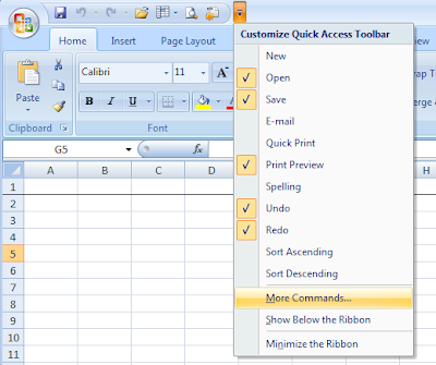
I continue to find new and frustrating things when using Excel 2007. For example, in most spreadsheets I want to freeze the top row and sometimes columns. To do this, I need to remember that I first need to go to the View Ribbon. If I want to use a Macro, it's not on the Insert or Data Ribbon, as I expected, but it is also on the View Ribbon. For Print Preview, you need to go to the Office Button and select the Print arrow. Needless to say, some of the most common tasks I perform are now hidden and/or further clicks away. One way to make some of these tasks easier is to use the new Quick Access Toolbar. The Quick Access Toolbar is the toolbar just right of the Office Button, above the Ribbons. By clicking the drop-down arrow to the right of the toolbar, you can customize the toolbar with your favorite shortcuts. Here's how to customize the Quick Access Toolbar. Click the drop-down arrow to the right of the Quick Access Toolbar Click on "More Commands...". This should ...

Word and Excel Hang on Startup

Perhaps it happened with prior versions of Word and Excel, but I definitely noticed for the first time switching to Office 2007. As a laptop user, I don't always work while connected to my office network, or it may just be that I'm connected via a much slower VPN connection. Regardless, every time I start Word and Excel, they ping the Default Printer, which happens to be on the office network. Due to this, whenever I'm using Word or Excel outside the office the applications hang for several minutes. Apparently so the onscreen display will match the Default Printer specifics, such as margins, Word and Excel will perform this action when started. When over 95% of my documents are never printed by me, and the great possibility that when printed by someone else, they won't have the same printer, I fail to see why Microsoft has chosen this path. From the research I've done, the workarounds are limited. For the Word/Excel VBA Power Users, you can write some code and have ...

Office Ribbon Frustrations: Switching Windows

I may be a little late to the party, but I finally upgraded to Office 2007 a few months back. While I like the new styles and themes, and I can still use the keyboard shortcuts I've learned, I'm still struggling with find other features within the Ribbons. Top of my list has been switching windows (view another open file) within Excel. In prior versions of Excel, I could go to the Windows menu and select another file. With Office 2007, you have to first select the View ribbon and then click Switch Windows, where you can select a different open file. As with many of the changes, I had to hunt for a while to find the Switch Windows option. In the mean time I did learn a new keyboard shortcut for switching windows. Use Ctrl-F6 or Ctrl-Shift-F6 to go in reverse order. As with the View >> Switch Windows menu, this also works in Word and PowerPoint as well as Excel.

Count the number of Rows after Auto-Filter in Excel

When you first apply an Auto-Filter in Excel, the Status Bar indicates the number of records in the filter (e.g. 517 of 8614). In many cases when you start performing other manipulations, the number disappears. Using a simple formula, you can calculate the filtered total. Assume you want to count all rows that are not empty -- the CountA function -- and assume you want to count the rows in column A. The formula would be SUBTOTAL(103,A:A)-1 . The syntax is as follows: subtotal(function_number, reference) , where function_number is 1 of many possible options as illustrated below. I included the "-1" to remove the count for the column heading row. function_num (includes hidden values) function_num (ignores hidden values) function 1 101 AVERAGE 2 102 COUNT 3 103 COUNTA 4 104 MAX 5 105 MIN 6 106 PRODUCT 7 107 STDEV 8 108 STDEVP 9 109 SUM 10 110 VAR 11 111 VARP Note: I used Excel 2003 for this example.

Clean imported Excel data

Sometimes when I get data from systems in CSV format, it includes a leading apostrophe ('). When viewing the data in a cell, the apostrophe does not appear, but when I look at it in the formula bar, it does. Without removing the leading apostrophe, any comparisons come up false. I tried removing the first character, but it removed the first displayed character. If you have a numeric field, you can divide the it by 1 (=c2/1), but that doesn't solve the problem for text fields. The solution is a built-in function Clean: =CLEAN(C2).

Create Hyperlinks in Excel Cells

Here's a simple trick. Some times I have data results in Excel, if combined with other URL data, it would take me to a specific record. For example, if I extracted Contact Record IDs from Salesforce.com and combined it with the URL prefix, I could view the record that corresponds to the ID. There are a few different approaches, but it all ends up using the same function: Hyperlink. Hyperlink takes two parameters: link_location and friendly_name (optional). Here are some examples: =HYPERLINK("https://na2.salesforce.com/" & B2) =HYPERLINK(CONCATENATE(A2, B2)) =HYPERLINK(CONCATENATE("https://na2.salesforce.com/", B2, C2)) =HYPERLINK("https://na2.salesforce.com/" & B2,"Joe Smith") The link location, in addition to being a URL could be a drive path (c:\foo\), a UNC path (\\Server1\folder1\), or even a "mailto:" (=HYPERLINK("mailto:" & H2)).

Excel displays formula instead of calculating

Here's a new one I just ran into. I entered a new formula into a cell, and it just displayed the formula, instead of calculating the results. It turns out the problem was due to the field being formatted as a Text field. Unfortunately, just by changing the field to a Number does not solve the problem. You must change the field to a Number and then re-enter the formula.

Copy a Formula down all the rows

Image
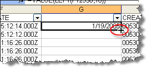
When working with large spreadsheets in Excel, it's very inefficient to copy the same formula down all the rows. Many of us already know that once we have our formula in our first row, we can drag the handle down to populate the remaining rows. But when we have 100s or even 1000s of rows, even this is not efficient. To allow Excel to do this for you, instead of dragging the handle, just double-click the handle. Here's the steps: Create formula in top cell Move cursor top lower-right corner of cell -- cursor should change to a plus (+) sign Double-click

Trim those cells in Excel

Image
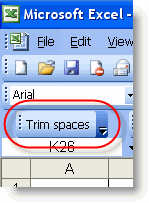
As I was working on a spreadsheet today, I realized that I had several cells with extra spaces at the end. I knew that there was a Trim function in Excel, but I didn't want to go through the hassle of determining the syntax and use, so instead I went to Google. THe third link I followed, I found Ablebits.com Trim Spaces for Microsoft Excel . Trim Spaces for Microsoft Excel is easy to install and easy to use, and works on many version of Excel. Here are the steps I followed: Downloaded Opened the zip file Opened the Readme.txt, which contained instructions Closed Excel Ran setup.exe Closed the Zip file Opened my Excel file in Excel Highlighted the cells to trim Clicked the Trim spaces button Saved my Excel file It doesn't get any easier! You can even use a silent installation -- great for IT groups who want to deploy. Ablebits.com Trim Spaces for Microsoft Excel is freeware, "The add-in is free for private and commercial use." That's a bargain, too. Here's are...

Use a Formula in an Excel Column, Bar, Line, or Pie Chart

Image
When you create Excel charts, you can populate the title with a formula. You might find this helpful to display a total quantity, such as in this example. Suppose you have 30 students and you are displaying their grade distribution in a pie chart. Here's what you do. Steps 1 - 4 set up the data; step 5 creates the Title formula; step 6 creates a pie chart. In the first column, skip the first line (A1) for the Title (we'll come back) In rows 2 - 6 of the first column (A2:A6), add the letter grades, A - D and F In column 2, rows 2 - 6 (B2:B6), add the number of grades of each type In column 2, row 7 (B7), sum the number of grades to get your student total Now go back to the first cell (A1) and add the following formula: ="Grade Distribution, " & B7 & " students" B7 is the same cell we put our total in, in step 4 If you want to format the value contained in B7m remember the TEXT functioned discussed in an earlier post Create your pie chart Highlight t...